Word Frequency Counter with R

2017-12-06

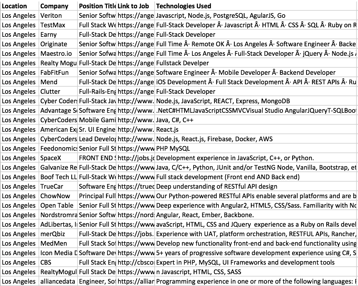
In the csv file below I wanted to find the top 10 most common technologies used in 30 job positions in Los Angeles. Instead of doing this manually I decided to use R. Below are the steps I took.

CSV FILE

Import the data into R

1
2
3
4
5
  #Make sure you are in the right working directory
  x = read.csv("focus.csv", stringsAsFactors=FALSE) #1
  data = data$Technologies.Used #2
  data = unlist(strsplit(data, "[ ]")) #3
  data = gsub(",","",data) #4

The first line above loads the csv file into R. I only want to look at the Technologies used column therefore I use line 2 to do just that. Line three unlist the data. Without this line we would be looking at rows instead of individual words. Line 4 removes all commas from each word.

Convert to lower case

1
 rdata = tolower(data)

Since R cannot recognize that “JavaScript” and “javascript” are the same word I converted all my words to lowercase.

Remove periods, blanks, and junk words

1
2
3
4
5
6
7
8
9
10
11
12
13
14
15
16
17
18
19
20
  removePeriod = which(data == "·")
  data = data[-removePeriod]

  removeBlanks = which(data == "")
  data = data[-removeBlanks]

  removeDeveloper = which(data == "developer")
  data = data[-removeDeveloper]

  removeExperience = which(data == "experience")
  data = data[-removeExperience]

  removeDevelopment = which(data == "development")
  data = data[-removeDevelopment]

  removeUsing = which(data == "using")
  data = data[-removeUsing]

  removeTime = which(data == "time")
  data = data[-removeTime]

I then cleaned up my data by removing periods from words, any empty strings in my data, and junk words. This method of removing words is fine for removing words that are uncommon. However, there is a much faster way of removing common words.

Remove common words

1
2
3
4
  url = "http://www.textfixer.com/resources/common-english-words.txt"
  stopwords= strsplit(readLines(url), ",")[[1]]
  removeWords=which(is.element(data, stopwords)==FALSE)
  data = data[removeWords]

I used the url above to find the most common english words. I then removed all common words from my data.

Plot the Graph

1
  barplot(sort(table(data))[(length(table(data))-10):length( table( data ) )], las=2, main = "Technology Focus in Los Angeles", ylab = "Frequency")

This last line of code is a bit heavy but basically it is creating a word frequency count of the cleaned data and graphing into a bar plot. This is the final output.

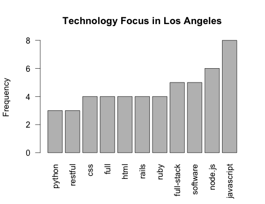
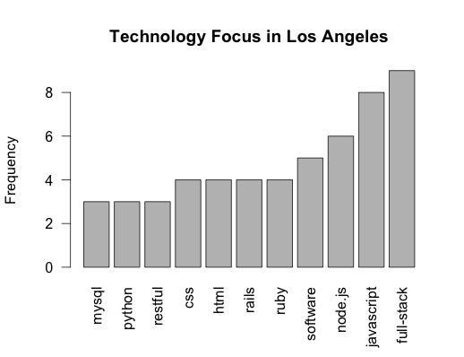
One thing to note is that R did not recognize “full” and “full-stack” were the same words. To fix this we can use gsub to replace “full” with “full-stack”

1
  data = gsub("(full)$","full-stack",data)

-dvcv